PIM_qtb
Purpose of Module
Module PIM_qtb generates trajectories according to one of the following stochastic methods:
These trajectories can be used to sample initial conditions for Linearized Semi-Classical Initial Value Representation (LSC-IVR) calculations.
Description of the module
The module implements different methods based on Langevin dynamics. The trajectories generated can be exploited directly or used to sample initial conditions for LSC-IVR calculations. The methods implemented are: classical Langevin dynamics, Quantum Thermal Bath (QTB) and two variants of adaptive QTB (adQTB-r and adQTB-f).
Classical Langevin dynamics
Classical Langevin dynamics is described by a stochastic differential equation :
(1)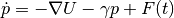
where  is the momentum vector of the set of
atoms, interacting via the potential
is the momentum vector of the set of
atoms, interacting via the potential  ,
,  is the damping coefficient
and
is the damping coefficient
and  is the stochastic force. The random force
is a Gaussian white noise: to enforce the classical fluctuation-dissipation theorem,
its autocorrelation spectrum is given by :
is the stochastic force. The random force
is a Gaussian white noise: to enforce the classical fluctuation-dissipation theorem,
its autocorrelation spectrum is given by :
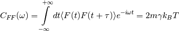
where  is the Boltzmann constant and
  the
temperature.
the
temperature.
Quantum Thermal Bath (QTB)
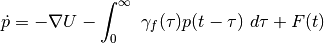
The Quantum Thermal Bath uses a generalized Langevin equation in order to approximate nuclear quantum effects [Dam] . In QTB dynamics, the stochastic force is no longer a white noise but is colored according to the following formula :
(2)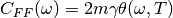
with
![\theta(\omega,T) = \hbar \omega \left[\frac{1}{2}+\frac{1}{e^{\hbar \beta \omega}-1}\right]](../../../_images/math/eb9930a905cdf8d5e012fb6f1edebe5cd2774378.png)
where  and
and  is the Planck
constant. The function
is the Planck
constant. The function  describes the energy
of a quantum harmonic oscillators of angular frequency
describes the energy
of a quantum harmonic oscillators of angular frequency
 at a temperature . The colored random force allows
approximating zero-point energy contributions to the equilibrium properties of the system.
The QTB method is known to lead to qualitatively
good results [Bri] but as many semi-classical methods, it suffers from zero-point energy leakage
(ZPEL) [Hern].
at a temperature . The colored random force allows
approximating zero-point energy contributions to the equilibrium properties of the system.
The QTB method is known to lead to qualitatively
good results [Bri] but as many semi-classical methods, it suffers from zero-point energy leakage
(ZPEL) [Hern].
Adaptive Quantum Thermal Bath (adQTB-r/f)
The Adaptive Quantum Thermal Bath is an extension of the QTB method, designed to eliminate the zero-point energy leakage by enforcing the energy distribution prescribed by the quantum fluctuation-dissipation theorem for each degree of freedom and each frequency, all along the trajectories [Man] .
In practice, this is done by minimizing the fluctuation-dissipation spectrum
 defined as:
(3)¶![\Delta_{FDT} (\omega) = {\rm{Re}} \left[C_{vF}(\omega)\right] - m \gamma_{r} (\omega) C_{vv} (\omega)](../../../_images/math/288c265f7c80c3287881bfca215ecbfa5a26496b.png)
where  is the velocity random force cross-correlation
spectrum,
is the velocity random force cross-correlation
spectrum,  the velocity autocorrelation spectrum and
 a set of damping coefficients dependent (or not) on
the frequency.
a set of damping coefficients dependent (or not) on
the frequency.
This minimization is carried out on the fly during the QTB simulation by dissymetrizing
the system-bath coupling coefficients corresponding to the damping force (dissipation)
and to the random force (energy injection).
This can be done either by directly modifying the random force spectrum
with frequency dependent damping term
 (adQTB-r variant) or by modifying the memory
kernel of the dissipative force
(adQTB-r variant) or by modifying the memory
kernel of the dissipative force  within the framework of a
non-Markovian generalized Langevin equation (adQTB-f variant).
within the framework of a
non-Markovian generalized Langevin equation (adQTB-f variant).
The coefficients  or
or  are slowly
adjusted with a first-order differential equation and an adaptation coefficient
are slowly
adjusted with a first-order differential equation and an adaptation coefficient
 :
:
(4)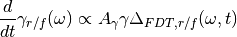
during a preliminary “adaptation time” until they reach convergence. Observables are then computed while the adaptive process is kept active. Further information and precise implementation details can be found in ref. [Man].
Two implementations are currently available in PaPIM:
Random force adaptive QTB (adQTB-r):
In this variant, the dissipation kernel is left unchanged, i.e.
 while the random force is modified according to a frequency-dependent
set of damping coefficients to satisfy
while the random force is modified according to a frequency-dependent
set of damping coefficients to satisfy
 (eq. (3)):
(5)

This method is applicable only if the initial damping coefficient
is large enough to compensate effects of a possible
zero-point energy leakage.Dissipative kernel adaptive QTB (adQTB-f)
In this approach, the random force is not modified, i.e.
 and remains the same as in the standard QTB
method (eq. (2))) but the dissipation term is not
described by a viscous damping term anymore (
and remains the same as in the standard QTB
method (eq. (2))) but the dissipation term is not
described by a viscous damping term anymore ( ) but
corresponds to a non-Markovian dissipative force. This leads to the following
generalized Langevin equation:
) but
corresponds to a non-Markovian dissipative force. This leads to the following
generalized Langevin equation:(6)
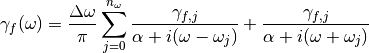
In order to avoid solving with brute force this integro-differential equation, the dissipative memory kernel is expressed as a sum of equally spaced (
 ) lorentzian functions of width
 :
:(7)
The parameter  are then modified to satisfy
(eq. (3)).
are then modified to satisfy
(eq. (3)).
Input file
To run PaPIM using one of the Langevin methods, one must set the parameter sampling_type in the sampling section to one of the following values:
- classical_langevin
- qtb
- adqtbr
- adqtbf
- dt : time step of the Langevin dynamics (REAL)
- lgv_nsteps : number of Langevin steps between each IVR sample (INTEGER)
- lgv_nsteps_therm : number of thermalization steps (INTEGER)
- integrator : integration method (two splitting methods are currently implemented: BAOAB, ABOBA (see reference [Lei] )) (STRING, default=“ABOBA”)
- damping : base damping coefficient for production runs
( in eq. :eq:eqLGV) (REAL)
- damping_therm : base damping coefficient for thermalization
( in eq. :eq:eqLGV) (REAL)
- qtb_frequency_cutoff : cutoff frequency for the QTB kernel (REAL)
- adqtb_agammas : (Only for adqtbr and adqtbf) adaptation speed
coefficient for adQTB ( in eq. (4))(REAL)
- adqtb_alpha : (Only for adqtbf) Width of the lorentzian used to
represent the dissipative kernel
 ( in eq. (7)) (REAL)
 - write_spectra : write average random force autocorrelation function ff, velocity autocorrelation function vv and velocity random force cross-correlation function vf spectra (LOGICAL, default=.FALSE.)
- write_trajectories : write Langevin trajectories in x,y,z,px,py,pz format (LOGICAL, default=.FALSE.)
Remark: all physical quantities are specified in Hartree atomic units.
Output files
The Langevin module is plugged to the IVR subroutines and thus can output the same correlation functions as the classical MC sampling. Additionally, it can write the Langevin trajectories and spectra obtained directly from them.
Langevin trajectories
If the parameter write_trajectories of the langevin section of the input file is set to TRUE, Langevin trajectories are saved. Trajectory files follow the following format:
num_of_atoms

    At_symbol(1)   X   Y   Z   Px  Py  Pz
    At_symbol(2)   X   Y   Z   Px  Py  Pz
       .
       .
    At_symbol(n)   X   Y   Z   Px  Py  Pz
num_of_atoms

    At_symbol(1)   X   Y   Z   Px  Py  Pz
    At_symbol(2)   X   Y   Z   Px  Py  Pz
       .
       .
    At_symbol(n)   X   Y   Z   Px  Py  Pz
 .
 .
 .
This corresponds to an extended XYZ format with information on momenta. It is readable by visualization software such as VMD to display the trajectories.
The module outputs multiple trajectory files depending on the number of independent trajectories (blocks) and the number of MPI processes. The naming follows the rules:
xp.traj.xyzfor 1 block and 1 processxp_proci.traj.xyzfor 1 block and multiple processesxp_proci_blockj.traj.xyzfor multiple blocks and processes
QTB analysis files
In addition to the trajectories, several files can be edited during the
simulations. They are useful to carefully check the convergence of the
adaptive QTB, notably by calculating  (eq. (3)).
ff_vv_vf_spectra.outspectra of random force and velocity autocorrelation and random force velocity cross-correlation functions (in atomic units) 


gamas.out(for adQTB-r and adQTB-f only) final set of optimized during the adaptive procedure (in atomic units)
Tests on implemented potentials
OH anharmonic potential
The classical Langevin has been tested on the OH anharmonic potential. The left panel of Figure Fig. 3 shows time correlation functions obtained with IVR using initial conditions sampled from classical (Boltzmann) Monte Carlo and from classical Langevin. Its right panel shows the corresponding spectra obtained by Fourier transform.
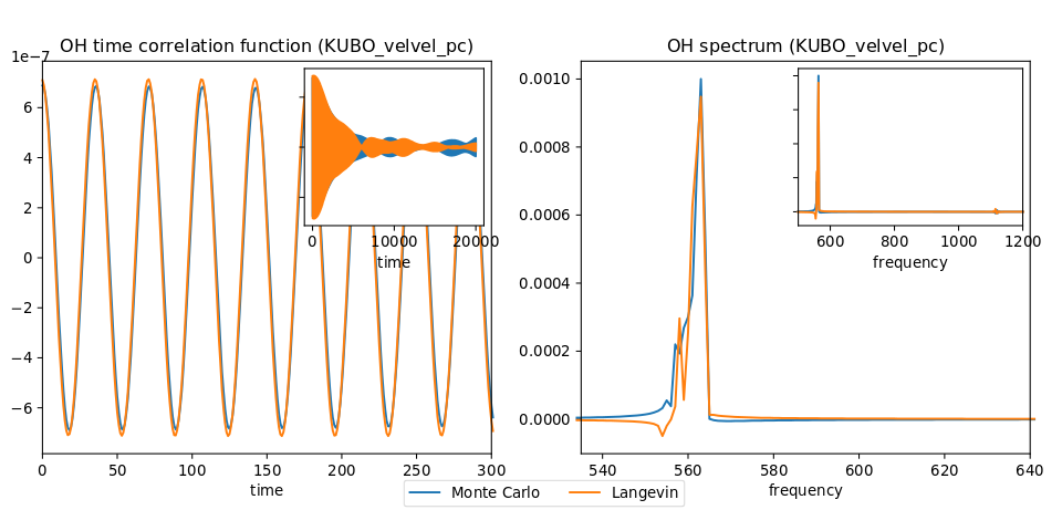
Fig. 3 Left panel: OH time correlation function using IVR with initial conditions sampled from MC and from Langevin. Right panel: corresponding spectra obtained by FFT.
Lennard-Jones  cluster
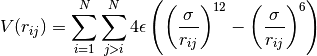
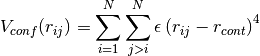
A Lennard-Jones potential has been implemented in
LennardJonesPot.f90 with the following pair potential:
(8)
A confining pair potential (useful in the cases of small clusters) can
be added to eq. (8). A 4th order polynomial is used for
distances greater than a chosen distance  :
:
(9)
Parameters for this potential are specified in an external text file. The file name is given in the input file using the parameter lennard_jones_parameters in section system. The parameters to specify are:
- epsil : depth of the potential well
 (in Kelvin)
(eq. (8))
(in Kelvin)
(eq. (8)) - sigma : distance for which the potential cancels
 (in
Å) (eq. (8))
(in
Å) (eq. (8)) - r_cont : minimum distance for which a confining potential
defined in eq. (9) is applied (in Å)
The QTB and both adaptive methods were tested on a Ne13 cluster in order
to reproduce results from reference [Man].
The Lennard-Jones parameters which have been used are
 ,
,  and
and  5 runs of
8000 steps with 16000 initial time steps are used with all four methods
(Langevin, QTB, adQTB-r,adQTB-f). Damping term is set to 5.0e-5 atomic
units and adaptive coefficients and for
adQTB-f to 5.0e-6 atomic units. Pair correlation function is then
computed from the trajectories output with a Python script
5 runs of
8000 steps with 16000 initial time steps are used with all four methods
(Langevin, QTB, adQTB-r,adQTB-f). Damping term is set to 5.0e-5 atomic
units and adaptive coefficients and for
adQTB-f to 5.0e-6 atomic units. Pair correlation function is then
computed from the trajectories output with a Python script
compute_g2r.py. Results are shown in figure Fig. 4 and are in
agreement with the ones of ref. [Man].
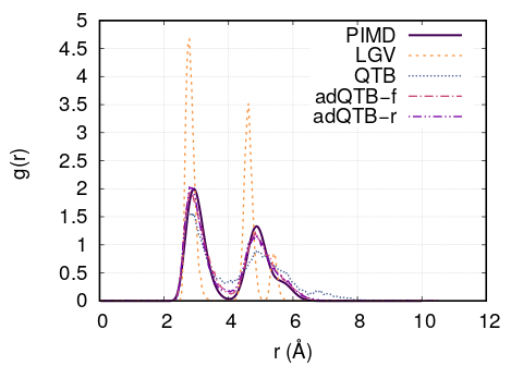
Fig. 4 Pair correlation function of Ne cluster obtained with
Langevin, QTB, adQTB-r and adQTB-f implemented with Langevin module
in PaPIM. Reference curve calculated with Path Integral Molecular
Dynamics (PIMD)
cluster obtained with
Langevin, QTB, adQTB-r and adQTB-f implemented with Langevin module
in PaPIM. Reference curve calculated with Path Integral Molecular
Dynamics (PIMD)
In this particular case, adaptive QTB leads to significantly better results than both classical Langevin and QTB when comparing them to the reference results obtained with PIMD (Path Integral Molecular Dynamics).
Implementation
Langevin module is built with the fewest modifications possible in the
main and previous code of PaPIM. The main program of the sampler is in
the file langevin.f90. It is structured in the same fashion as the
existing samplers (PIM.f90 and ClassMC.f90) and only provides
the subroutine langevin_sampling to the main program.
Source files
The Langevin module is divided in multiple files:
langevin.f90: contains the Langevin sampler and links the main code with the other files of the modulelangevin_integrator.f90: subroutines to integrate Langevin equationslangevin_analysis.f90: spectral analysis tools for Langevin and (ad)QTB trajectoriesqtb_random.f90: generation of QTB colored noise and adaptation subroutines for adQTB
Other modifications
Some other routines have been modified during the implementation of Langevin module.
PaPIM.f90: main code ; add calls to Langevin moduleGlobType.f90: add declarations for LangevinReadFiles.f90: read input files
Compiling
A Fortran 90/95 compiler with MPI wrapper is required for successful compilation
of the code.
Although the correlation function subroutines are serial, the remaining code is
parallelized so MPI wrappers have to be used.
The code must be compiled using the FFTW library.
Quantum correlation subroutines within PIM_qtb modules are compiled by executing
the command make in the ./source directory.
The same make command generates a PaPIM.exe executable for testing of the correlation functions.
Testing
For PIM_qtb test purposes the numdiff package is used for automatic comparison purposes and should be made
available before running the tests, otherwise the diff command will be used automatically instead but the user
is warned that the test might fail due to numerical differences.
The user is advised to download and install numdiff from here.
Tests and corresponding reference values are located in sub-directories ./tests/xxx, where xxx stands
for oh and lj systems.
lj tests also requires a Python distribution.
Before running the tests the code has to be properly compiled by running the make command in the
./source sub-directory:
Tests can be executed automatically by running the command in the ./tests sub-directory :
#. ./test+lgv.sh for tests on OH bonds compared to previous classical implementation
#. ./test_lj.sh for tests on a Ne:.
All test are executed on one processor core.
Due to small numerical discrepancies between generated outputs and reference values which
can cause the tests to fail, the user is advised to manually examine the numerical differences
between generated output and the corresponding reference values in case the tests fail.
Source Code
The PIM_qtb module source code is located at: https://gitlab.e-cam2020.eu:10443/thomas.ple/PIM.git (Temporary link).
Source Code Documentation
The documentation can also be compiled by executing the following commands
in ./doc/QTB_doc directory with “Sphinx” (documentation tool) python module installed:
sphinx-build -b html source build
make html
The source code documentation can be generated automatically in ./doc sub-directory,
html and latex format, by executing the following command in the ./doc directory:
doxygen PIMqcf_doxygen_settings
References
| [Dam] | (1, 2) H. Dammak, Y. Chalopin, M. Laroche, M. Hayoun, J.-J. Greffet, Quantum Thermal Bath for Molecular Dynamics Simulation, Phys. Rev. Lett. 103 (2009) 190601. |
| [Man] | (1, 2, 3, 4, 5) E. Mangaud, S. Huppert, T. Plé, P. Depondt, S. Bonella, F. Finocchi, The Fluctuation–Dissipation Theorem as a Diagnosis and Cure for Zero-Point Energy Leakage in Quantum Thermal Bath Simulations, J. Chem. Th. Comput. 15 (2019) 2863-2880. |
| [Bri] | F. Brieuc, Y. Bronstein, H. Dammak, P. Depondt, F. Finocchi, M. Hayoun, Zero-point energy leakage in quantum thermal bath molecular dynamics simulations, J. Chem. Th. Comput. 12 (2016) 5688–5697. |
| [Hern] | J. Hern’andez-Rojas, F. Calvo, E. G. Noya, Applicability of Quantum Thermal Baths to Complex Many-Body Systems with Various Degrees of Anharmonicity, Journal of Chemical Theory and Computation 11 (2015) 861–870. |
| [Lei] | B. Leimkuhler, C. Matthews, Rational Construction of Stochastic Numerical Methods for Molecular Sampling, Applied Mathematics Research eXpress (2012). |