G-CTMQC¶

Purpose of Module
Background Information
Building and Testing
Source Code
References

Studies in the domain of photochemistry and photophysics strongly rely on simulation methods able to describe strong coupling between electronic and nuclear motion on the femtosecond time scale, usually called nonadiabatic coupling. Simulations give access to microscopic information in terms of molecular structures, electronic populations, vibrational energies that can be easily compared to experiments, for instance in the domains of time-resolved spectroscopy or 2D spectroscopy. In addition to this, molecular dynamics simulations allow to follow in real time the evolution of molecular systems, thus providing support to interpret and even predict the outcome of experiments.

Photochemical and photophysical reactions are ubiquitous in nature, from photosynthesis to vision, and are more and more exploited for technological advances, as for the photo-current production in organic photovoltaic devices. In addition, it is becoming clear the importance to consider spin-orbit coupling even in those systems composed of light elements, such as oxygen and carbon, to be able to describe processes such as intersystem crossings in organic light-emitting diodes.

G-CTMQC module provides numerical tools to perform simulations of internal conversion (spin-allowed) and intersystem crossing (spin-forbidden) phenomena underlying photochemical and photophysical reactions. G-CTMQC gives the user the flexibility of employing different approaches and, thus, various approximation schemes, to achieve dynamical information as accurate as possible, as well as ample flexibility in the choice of systems that be studied thanks to the interface of G-CTMQC with QuantumModelLib (E-CAM module).

Purpose of Module ¶

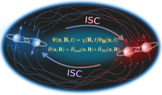
G-CTMQC is a module for excited-state molecular dynamics simulations with various trajectory-based algorithms, including nonadiabatic coupling and spin-orbit coupling. Nuclear dynamics can be performed based on the quantum-classical algorithm derived from the exact factorization of the electron-nuclear wavefunction [EF], dubbed CT-MQC [CT-MQC]. Recently, the extension of the exact-factorization theory has been proposed to include spin-orbit coupling [SOC]. Therefore, the “generalized” algorithm is now able to treat (i) standard nonadiabatic situations, where spin-allowed electronic transitions among states with the same spin multiplicity are mediated by the coupling to nuclear motion, and (ii) spin-orbit interactions, where spin-forbidden electronic transitions among states of different spin multiplicity are induced by the spin-orbit coupling.

Electronic evolution is carried out in the adiabatic basis for standard nonadiabatic problems. In the case of spin-orbit interactions, G-CTMQC offers the options to use the spin-diabatic or the spin-adiabatic representations. Information about electronic-structure properties, ie, energies, gradients and couplings, is calculated and read on-the-fly at the positions of the trajectories at each time step based on the QuantumModelLib library [4] of potentials (which G-CTMQC is interfaced to).

In addition, the code offers the possibility of performing calculations with the trajectory surface hopping algorithm [TSH] and the Ehrenfest approach [EH]. Concerning the trajectory surface hopping method, the fewest switches scheme is implemented, along with the energy decoherence corrections to fix the overcoherence issue of surface hopping [TSH-EDC]. For surface hopping and Ehrenfest, only nonadiabatic couplings are currently implemented.

Background Information ¶

Detailed information about the exact factorization and CT-MQC [EF] can be found in CTMQC where the original version of the module is described. The generalized CTMQC, G-CTMQC, includes various new features to original module:

spin-allowed, between electronic states of the same spin multiplicity, and spin-forbidden, between electronic states of different spin multiplicity, transitions can be simulated; the former are mediated by the kinetic, also called nonadiabatic, coupling between electronic and nuclear motion, whereas the latter are induced by spin-orbit coupling;
G-CT-MQC calculations, based on the generalized coupled-trajectory mixed quantum-classical algorithm, can be performed in the spin-diabatic and spin-adiabatic basis for the electronic subsystem;
nonadiabatic calculations based on trajectory surface hopping [TSH] and on the Ehrenfest approach [EH] can be carried out, including energy decoherence corrections in surface hopping [TSH-EDC]; the fewest switches scheme is used for surface hopping;
on-the-fly dynamics can be performed based on the calculation of electronic structure information, namely energies, gradients and couplings, along the trajectories via the interface to the QuantumModelLib library.

The new features introduced in G-CTMQC are documented in Refs. [SOC] and [G-CT-MQC] concerning the inclusion of spin-orbit coupling in the exact factorization and in G-CTMQC, in Refs. [PSB3] and [IC] concerning the inclusion of trajectory surface hopping, Ehrenfest dynamics, and different possibilities of sampling the initial conditions.

Building and Testing ¶

G-CTMQC is a fortran90 based code. Compilation of the code requires the gfortran compiler, and Lapack libraries. Tests have been performed with GCC 7.x. Note that, before compiling G-CTMQC it is necessary to compile the potential library available here and copy the file libpot.a into the src directory of G-CTMQC.

Once the main directory CTMQC has been downloaded, go to the directory and

cd ./src

make

Running the command make will compile the source code and generate the executable main.x. Go back to the CTMQC directory with the command

cd ../

and run the script

./create_dirs.sh

that creates the directory output where all output files will be generated. Notice that you should run this script in each new directory where you run the executable. The program generates a series of output files that are saved in different directories. Therefore, in order not to obtain errors during the execution of the program, the directories have to be created.

CREATE THE OUTPUT DIRECTORY

The directory output contains several subdirectories. After successful execution of the program, those subdirectories will contain $N_{\textrm{files}} = N_{\textrm{steps}}/N_{\textrm{dump}}$ files, with $N_{\textrm{steps}}$ the number of total time steps and and $N_{\textrm{dump}}$ the number of time steps after which a new output file is generated. In each subdirectory, the files are labelled with an index increasing with time, from 0 to $N_{\textrm{files}}$ . In the current version of the code, up to 999 files can be created.

The following subdirectories of the directory output will be created.

coeff

Each file (named coeff.xxx.dat) in this directory contains the coefficients $C_k^{(I)}(t)$ of the expansion of the electronic wavefunction in the used electronic basis as a function of the position of the corresponding trajectory $I$ . Each file is in the form: the first $N_{\textrm{dof}}$ columns are the positions of the trajectories for each of the $N_{\textrm{dof}}$ nuclear degrees of freedom; the following n x n columns are the real parts of $[C_k^{(I)} (t)]^*[C_l^{(I)}(t)]$ with $k,l=1,n$ and $n$ the number of electronic states considered in the expansion; the following n x n columns are the imaginary parts of $[C_k^{(I)} (t)]^*[C_l^{(I)}(t)]$ with $k,l=1,n$ .

histo:  [only for one-dimensional calculations]

Each file (named histo.xxx.dat) in this directory contains the nuclear density approximated as a histogram that is constructed from the distribution of classical trajectories. The data listed in the file have the form: first column the position along the nuclear coordinated (coarser that the original grid, but defined in the same domain); second column the normalized histogram.

trajectories

Each file (named RPE.xxx.dat) in this directory contains the values of the phase-space variables and the value of the gauge-invariant part of the time-dependent potential energy surface. The data listed in the file have the form: the first $N_{\textrm{dof}}$ columns are the positions of the trajectories for each of the $N_{\textrm{dof}}$ nuclear degrees of freedom; the following $N_{\textrm{dof}}$ columns are the momenta of the trajectories for each of the $N_{\textrm{dof}}$ nuclear degrees of freedom; the following column is the gauge-invariant part of the time-dependent potential energy surface; the following $n$ columns are the adiabatic energies.

Additionally, the files BO_population.dat and BO_coherences.dat are created, containing the population of the adiabatic states and the indicator of coherence as functions of time (the first columns is the time in atomic units). They are defined as

$\rho_k(t) = \frac{1}{N_{traj}}\sum_{I=1}^{N_{traj}} \left|C_k^{(I)}(t)\right|^2$

and

$\eta_{kl}(t) = \frac{1}{N_{traj}}\sum_{I=1}^{N_{traj}} \left|C_k^{(I)}(t)C_l^{(I)}(t)\right|^2$

respectively, with $k=1,\ldots,n$ .

PROVIDED TESTS AND INPUT FILE

In the main CTMQC directory the

tests

directory provides examples of input files to run one-dimensional calculations with CT-MQC, surface hopping and Ehrenfest on Tully model #3 [TSH] and some reference calculations.

  &SYSTEM
   TYP_CAL            = "XX"       !*character* XX = CT (CT-MQC calculations), EH (Ehrenfest calculations), SH (surface hopping calculations)
   SPIN_DIA           = X          !*logical* X = T only for calculations with spin-orbit coupling in the spin-diabatic basis, otherwise X = F
   NRG_CHECK          = X          !*logical* X = T to switch off the spin-orbit coupling when the energy between states is larger than NRG_GAP
   NRG_GAP            = X          !*real* only for calculations with spin-orbit coupling in the spin-diabatic basis
   MODEL_POTENTIAL    = "XXXXX"    !*character* XXXXX = definition of the model as it appears in QuantumModelLib
   OPTION             = X          !*integer* X = 1, 2, 3 for Tully's models #1, #2, #3 (only used for Tully's models calculations)
   N_DOF              = X          !*integer* X = number of nuclear degrees of freedom
   PERIODIC_VARIABLE  = X,X,X...   !*logical* one value for each nuclear degree of freedom with X = T (periodic coordinate) or F
   PERIODICITY        = X,X,X...   !*real* one value for each nuclear degree of freedom with X = the period in units of PI
   NSTATES            = X          !*integer* X = number of electronic states
   M_PARAMETER        = X,X,X...   !*real* one value for each nuclear degree of freedom with X = typical distance to tune the coupling among the trajectories in CT calculations
   QMOM_FORCE         = X          !*logical* X = F to switch off the force from the quantum momentum (only) in CT calculations
   DECOHERENCE        = X          !*logical* X = F for surface hopping or T for surface hopping with energy decoherence corrections
   C_PARAMETER        = X          !*real* energy parameter for the energy decoherence correction in surface hopping
   JUMP_SEED          = X          !*integer* seed for random number generator for the hopping algorithm in SH calculation
 /

 &DYNAMICS
  FINAL_TIME       = X             !*real* X = length of the simulation in atomic units
  DT               = X             !*real* X = integration time step in atomic units
  DUMP             = X             !*integer* X = number of time steps after which the output is written
  INITIAL_BOSTATE  = X             !*integer* X = initial electronic state
  NTRAJ            = X             !*integer* X = number of classical trajectories
  R_INIT           = X,X,X...      !*real* one value for each nuclear degree of freedom with X = average position of the initial nuclear distribution
  K_INIT           = X,X,X...      !*real* one value for each nuclear degree of freedom with X = average momentum of the initial nuclear distribution
  SIGMAR_INIT      = X,X,X...      !*real* one value for each nuclear degree of freedom with X = variance in position space of the initial nuclear distribution
  SIGMAP_INIT      = X,X,X...      !*real* one value for each nuclear degree of freedom with X = variance in momentum space of the initial nuclear distribution
  MASS_INPUT       = X,X,X...      !*real* one value for each nuclear degree of freedom with X = the nuclear mass
/

&EXTERNAL_FILES
 POSITIONS_FILE     = "XXXXX"      !*character* XXXXX = file containing the list of initial positions for the trajectories; if the field is empty, positions are sampled according to R_INIT and SIGMAR_INIT
 MOMENTA_FILE       = "XXXXX"      !*character* XXXXX = file containing the list of initial momenta for the trajectories; if the field is empty, momenta are sampled according to K_INIT and SIGMAP_INIT
 OUTPUT_FOLDER      = "XXXXX"      !*character* XXXXX = path to the location where the output is written
/

Source Code ¶

The G-CTMQC source code and test files can be found following this link.

References ¶

[EF]	(1, 2) F. Agostini, E. K. U. Gross, Quantum chemistry and dynamics of excited states: Methods and applications, edited by L. González and R. Lindh, Wiley (2020).

[CT-MQC]

S. K. Min, F. Agostini, E. K. U. Gross, Phys. Rev. Lett. 115 (2015) 073001 DOI: 10.1103/PhysRevLett.115.073001

[TSH]

(1, 2, 3) J. C. Tully, J. Chem. Phys. 93 (1990) 1061 DOI: 10.1063/1.459170

[EH]	(1, 2) J. C. Tully, Faraday Discuss. 110 (1998) 407 DOI: 10.1039/A801824C

[TSH-EDC]

(1, 2) G. Granucci, M. Persico, J. Chem. Phys. 126 (2007) 134114 DOI: 10.1063/1.2715585

[G-CT-MQC]

F. Talotta, S. Morisset, N. Rougeau, D. Lauvergnat, F. Agostini, J. Chem. Theory Comput. 16 (2020) 4833-4848 DOI: 10.1021/acs.jctc.0c00493

[PSB3]

E. Marsili, M. Olivucci, D. Lauvergnat and F. Agostini, J. Chem. Theory Comput. 16 (2020) 6032-6048 DOI: 10.1021/acs.jctc.0c00679

[SOC]

(1, 2) F. Talotta, S. Morisset, N. Rougeau, D. Lauvergnat, F. Agostini, Phys. Rev. Lett. 124 (2020) 033001 DOI: 10.1103/PhysRevLett.124.033001

[IC]	C. Pieoroni, E. Marsili, D. Lauvergnat and F. Agostini, J. Chem. Phys. 154 (2021) 034104 DOI: 10.1063/5.0036726

G-CTMQC¶

Purpose of Module¶

Background Information¶

Building and Testing¶

Source Code¶

References¶

Purpose of Module ¶

Background Information ¶

Building and Testing ¶

Source Code ¶

References ¶