Particle Insertion Core¶

Purpose of the Module
Background Information
General Formulation
Algorithms
Source Code
Compilation and Linking
Scaling and Performance

Purpose of the Module ¶

This software module computes the change in free energy associated with the insertion or deletion of Lennard Jones particles in dilute or dense conditions in a variety of Thermodynamic Ensembles, where statistical sampling through molecular dynamics is performed under LAMMPS but will be extended to other molecular dynamics engines at a later date. Lennard-Jones type interactions are the key source of difficulty associated with particle insertion or deletion, which is why this module is a core module, as other interactions including Coulombic and bond, angle and dihedral interactions will be added in a second module. It differs from the main community approach used to date to compute such changes as it does not use soft-core potentials. Its key advantages over soft-core potentials are: (a) electrostatic interactions can in principle be performed simultaneously with particle insertion (this and other functionalities will be added in a new module); and, (b) essentially exact long-range dispersive interactions using dispersion Particle Mesh Ewald (PMME) or EWALD if desired can be selected at runtime by the user.

Background Information ¶

Particle insertion can be used to compute the free energy associated with hydration/drying, the insertion of cavities in fluids/crystals, changes in salt levels, changes in solvent mixtures, and alchemical changes such as the mutation of amino-acids. in crystals. It can also be used to compute the free energy of solvent mixtures and the addition of salts, which is used in the purification processing industrially, for instance in the purification of pharmaceutical active ingredients. Particle insertion can in principle also be used to compute the free energy associated with changes in the pH, that is the proton transfer from a titratable site to the bulk, for example in water.

Our approach consists of rescaling the effective size of inserted atoms through a parameter $\lambda$ so that all interactions between nserted atoms and interactions between inserted atoms and atoms already present in the system are zero when $\lambda = 0$ , creating at most an integrable singularity which we can safely handle. In the context of Lennard-Jones type pair potentials, our approach at a mathematical level is similar to Simonson, who investigated the mathematical conditions required to avoid the singularity of insertion. It turns out that a non-linear dependence of the interaction on :math:’lambda’ between inserted atoms and those already present is required (i.e. a simple linear dependence on :math: ‘lambda’ necessarily introduces a singularity).

This module and upcoming modules include computing the free energy changes associated with the following applications

hydration and drying;

the addition of multiple molecules into a condenses environment;

residue mutation and alchemy;

constant pH simulations, this also will also exploit modules created in E-CAM work package 3 (quantum dynamics); and,

free energy changes in chemical potentials associated with changes in solvent mixtures.

General Formulation ¶

Consider a system consisting of $N+M$ degrees of freedom and the Hamiltonian

$H(r,p,\lambda) =&H_0 + KE_{insert} + \Delta V(r, \lambda)$

where $H_0$ corresponds to an unperturbed Hamiltonian, and the perturbation $\Delta V(r, \lambda)$ depends nonlinearly on a control parameter $\lambda$ . The first set of N degrees of freedom is denoted by A and the second set of M degrees of freedom is denoted by B. To explore equilibrium properties of the system, thermostats, and barostats are used to sample either the NVT (canonical) ensemble or the NPT (Gibbs) ensemble. The perturbation is devised so that when $\lambda = 0$ , $\Delta V(r, \lambda) = 0$ , B is in purely virtual. When $\lambda = 1$ , B corresponds to a fully physical augmentation of the original system.

In the present software module, we consider only interaction Lennard Jones atoms.

$\Delta V(r,\lambda) = V_{lj}(r,\lambda)$

where for each inserted atom i

$\hat{\sigma}( \lambda)_i &= \lambda \sigma_i \\ \hat{\epsilon}( \lambda)_i &= \lambda \epsilon_i \\$

and the mixing rule for Van der Waals diameters and binding energy between different atoms uses the geometric mean. The dependence of $\sigma$ on $\lambda$ has the consequence that the mean $\sigma$ between a pair of inserted atoms scales as $\lambda$ , but scales as $\sqrt{\lambda}$ when one atom in the pair is inserted and the other is already present. These choices of perturbations guarantees that the particle insertion and deletion catastrophes are avoided.

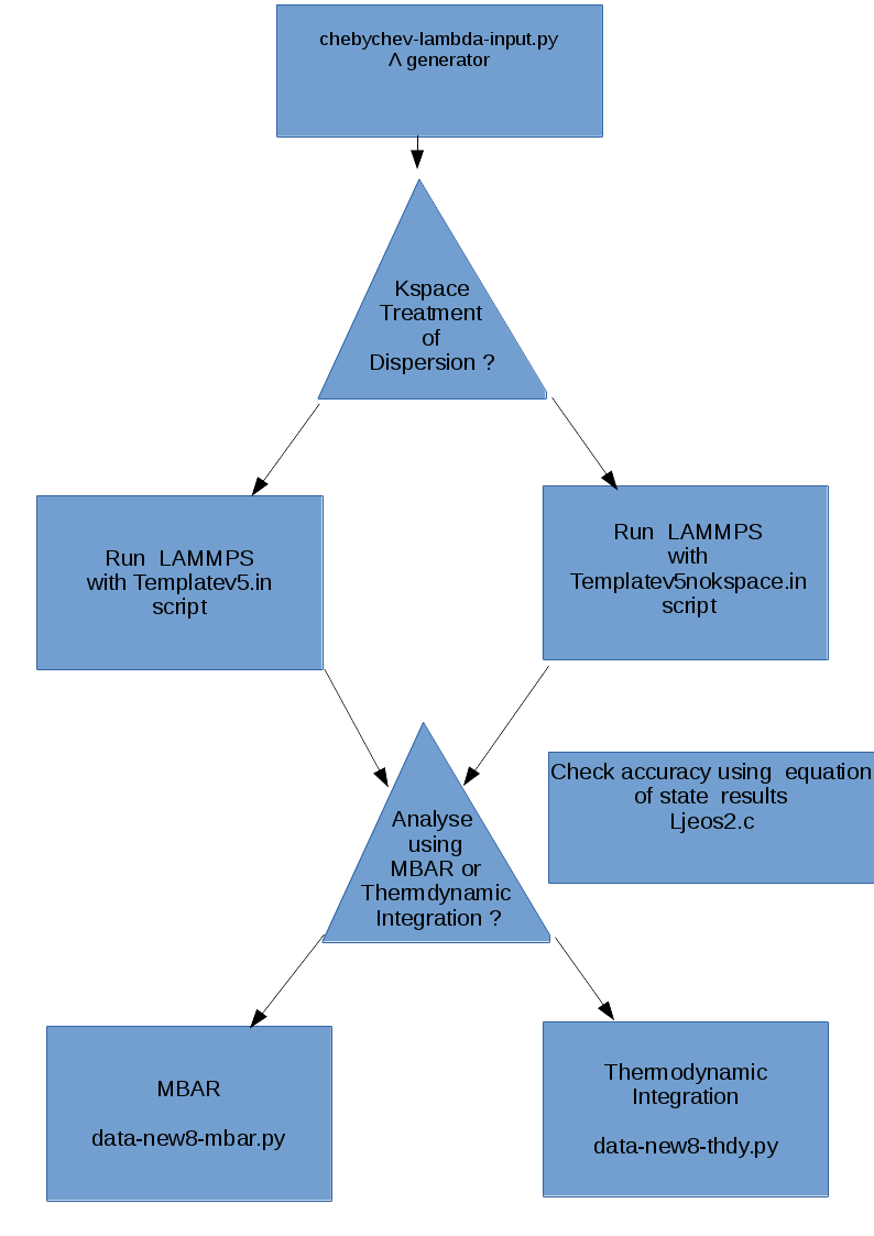
Algorithms ¶

At the core of the PI core module there are four functions/codes. The first written in python generates the interpolation points which are the zero’s of suitably transformed Chebyshev functions.

The second code written ln LAMMPS scripting language performs the simulation in user-defined ensembles at the selected interpolation values of :math:’lambda’, at a user-specified frequency, computing two-point central difference estimates of derivatives of the potential energy needed for thermodynamic integration, computing the energy functions for all values of :math:’lambda’ in the context of MBAR. The user also specifies the locations of the inserted particles. The user also specifies whether Particle Mesh Ewald or EWALD should be used for dispersive interactions.

The third code written in python takes the output data from LAMMPS, prepares it so that free energy differences in the selected ensemble can be computed using MBAR provided by the pymbar suite of Python codes of the Chodera group.

The fourth code, also written in python take the LAMMPS output and performs the thermodynamic integration.

Source Code ¶

All files can be found in the PIcore subdirectory of the particle_insertion git repository.

Compilation and Linking ¶

See PIcore README for full details.

Scaling and Performance ¶

As the module uses LAMMPS, the performance and scaling of this module should essentially be the same, provided data for thermodynamic integration and MBAR are not generated too often, as is demonstated below. In the case of thermodynamic integration, this is due to the central difference approximation of derivatives, and in the case of MBAR, it is due to the fact that many virtual moves are made which can be extremely costly if the number of interpolating points is large. Also, when using PMME, the initial setup cost is computationally expensive, and should, therefore, be done as infrequently as possible. A future module in preparation will circumvent the use of central difference approximations of derivatives. The scaling performance of PI-CORE was tested on Jureca multi node. The results for weak scaling (where the number of core and the system size are doubled from 4 to 768 core) are as follows.

Weak Scaling:

Number of MPI Core	timesteps/s
4	1664.793
8	1534.013
16	1458.936
24	1454.075
48	1350.257
96	1301.325
192	1263.402
384	1212.539
768	1108.306

and for the strong scaling (where the number of core are doubled from 4 to 384 but the system size is fixed equal to 768 times the original system size considered for one core/processor for weak scaling) Strong Scaling:

Number of MPI Core	timesteps/s
4	9.197
8	17.447
16	34.641
24	53.345
48	104.504
96	204.434
192	369.178
384	634.022

Particle Insertion Core¶

Purpose of the Module¶

Background Information¶

General Formulation¶

Algorithms¶

Source Code¶

Compilation and Linking¶

Scaling and Performance¶